TinyML Vibration Research Reproduction
- ESP32-S3 (N8R8)
- MPU6050 IMU
- SH1106 OLED
- I²C Protocol
- Complementary Filter
- Direct Register Access
- C/C++
- 3D Projection
TinyML Research Reproduction: Part 1 · Hardware & Sensor Validation
Building the physical foundation for embedded vibration anomaly detection: validating the sensing layer, overcoming unexpected register responses, implementing sensor fusion, and rendering real-time 3D telemetry on an ESP32-S3.
⚡ Project Overview
In industrial environments, unexpected mechanical failures in motors, pumps, and rotating machinery lead to costly downtime. Modern predictive maintenance increasingly relies on TinyML—running lightweight machine learning inference directly on resource-constrained microcontrollers at the edge.
This project is the first stage of my research reproduction of an embedded anomaly detection system designed to monitor and detect abnormal motor vibrations. The reference research utilizes an MPU6050 inertial measurement unit (IMU) to capture physical vibration signals, which are then processed by an on-device microcontroller prior to machine-learning classification.
Rather than treating the machine learning model as a black box and jumping straight to training, I adopted a hardware-upward methodology:
Sensor ──> Data ──> Signal Understanding ──> Processing ──> TinyML
Before an embedded model can classify anomalies, the physical data stream feeding it must be dependable, calibrated, and well understood. Part 1 focuses entirely on this foundation: establishing robust hardware communication, debugging sensor behavior at the register level, implementing sensor fusion, and building a real-time visual telemetry pipeline on a 128×64 OLED display.
🛠️ Hardware Setup & Architecture
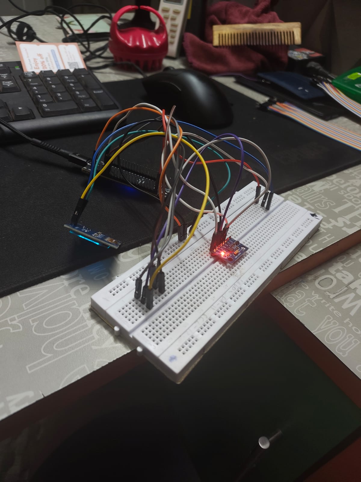
The prototype is constructed on a solderless breadboard around the ESP32-S3 N8R8 microcontroller, an MPU6050 6-DOF IMU, and a 1.3-inch 128×64 SH1106 monochrome OLED display.
| Parameter | Specification | Details |
|---|---|---|
| Microcontroller | ESP32-S3 N8R8 | Dual-core Xtensa® 32-bit LX7 @ 240 MHz, 8 MB Flash, 8 MB PSRAM |
| Motion Sensor | MPU6050 | 3-axis accelerometer + 3-axis gyroscope with integrated 16-bit ADCs |
| Display Panel | 1.3" Monochrome OLED | 128 × 64 pixels, SH1106 driver controller |
| Communication Bus | I²C (Shared 2-Wire) | Single shared bus operating at 3.3V logic levels |
| MPU6050 Address | 0x68 | Configured via AD0 pulled low to GND |
| OLED Address | 0x3C | Standard monochrome display driver address |
| Serial Data (SDA) | GPIO 11 | Shared I²C data line |
| Serial Clock (SCL) | GPIO 12 | Shared I²C clock line |
| Supply Voltage | 3.3V DC | Powered from the ESP32-S3 regulated 3.3V rail |
🔌 Pinout & Bus Interconnect
Both the MPU6050 sensor and the SH1106 OLED display share the primary hardware I²C bus of the ESP32-S3, keeping pin usage minimal:
+-------------------------------------------------------------+
|                     ESP32-S3 N8R8 Board                     |
|                                                             |
|   3.3V Out    GND         GPIO 11 (SDA)     GPIO 12 (SCL)   |
+------|---------|----------------|-----------------|---------+
       |         |                |                 |
       +---------+-------+        |                 |
       |         |       |        |                 |
+------v---------v-------v--------v-----------------v---------+
|                  Shared I²C Breadboard Bus                  |
+------|---------|----------------|-----------------|---------+
       |         |                |                 |
       |  +------+                |                 |
       |  |                       |                 |
+------v--v-----------------------v-----------------v---------+
|  VCC   GND   AD0(->GND)        SDA               SCL        |
|  MPU6050 6-DOF IMU (I2C: 0x68)                             |
+-------------------------------------------------------------+
       |  |                       |                 |
+------v--v-----------------------v-----------------v---------+
|  VCC   GND                     SDA               SCL        |
|  1.3" SH1106 OLED Display (I2C: 0x3C)                       |
+-------------------------------------------------------------+
Connection Mapping Table
| Device Pin | ESP32-S3 Connection | Function / Description |
|---|---|---|
| MPU6050 VCC | 3.3V | 3.3V DC system power |
| MPU6050 GND | GND | Common ground reference |
| MPU6050 SDA | GPIO 11 | I²C Serial Data line |
| MPU6050 SCL | GPIO 12 | I²C Serial Clock line |
| MPU6050 AD0 | GND | Sets 7-bit slave address to 0x68 |
| OLED VCC | 3.3V | 3.3V DC system power |
| OLED GND | GND | Common ground reference |
| OLED SDA | GPIO 11 | I²C Serial Data line |
| OLED SCL | GPIO 12 | I²C Serial Clock line |
🔍 Sensor Validation & Direct Register Access
Before implementing signal processing or machine learning inference, the sensor must communicate reliably and return valid physical measurements.
An initial I²C bus scan successfully verified that the MPU6050 was responding at address 0x68. However, when attempting initialization via standard high-level MPU6050 Arduino libraries, the driver failed and reported the device as unavailable.
The WHO_AM_I Register Anomaly
Investigating the failure at the register level revealed the root cause:
- Standard MPU6050 devices return
0x68when querying theWHO_AM_Iregister (0x75). - High-level libraries perform a strict sanity check:
if (readRegister(0x75) != 0x68) fail(); - In my prototype setup, the sensor reliably returned:
WHO_AM_I = 0x70
Because of this mismatch, the library threw an error and refused to proceed. However, inspecting the configuration and measurement registers demonstrated that the silicon was fully operational:
- Writing to
PWR_MGMT_1(0x6B) successfully woke the device from sleep mode. - The accelerometer registers (
0x3Bto0x40) produced clean, responsive raw counts. - The gyroscope registers (
0x43to0x48) responded accurately to rotational motion.
Rather than relying on brittle library abstractions, I switched to direct register communication over the ESP32-S3 I²C bus: configuring the power management registers, setting full-scale ranges, and polling the high and low data bytes directly.
📐 Understanding the Motion Data
The MPU6050 provides two complementary categories of physical information:
- 3-Axis Accelerometer ($a_x, a_y, a_z$): Measures total linear acceleration including the earth's static gravity vector ($1g \approx 9.81\text{ m/s}^2$).
- 3-Axis Gyroscope ($\omega_x, \omega_y, \omega_z$): Measures angular rate of change (angular velocity in degrees or radians per second).
Understanding this physical distinction proved essential when translating sensor readings into motion visualization.
🐛 The Debugging Milestone: The Perpetually Rotating Cube
My first prototype for visualizing motion mapped the accelerometer readings directly into cumulative rotation angles for a 3D wireframe cube.
While moving the breadboard dynamically, the visual response appeared convincing. However, as soon as the breadboard was set stationary on the workbench, an immediate flaw surfaced: the cube kept rotating continuously without stopping.
    Stationary Sensor
           │
           ▼
Measures 1g Gravity Vector
           │
           ▼
Accumulated into Rotation Angle (naive loop)
           │
           ▼
Cube continues spinning endlessly!
A stationary accelerometer does not measure zero; it continuously measures the static gravity vector pointing downward. By integrating or continuously accumulating raw acceleration values as angular displacement, the software was constantly instructing the rendering loop to turn.
This highlighted a fundamental rule of inertial sensing:
Acceleration is not the same thing as rotation.
Visualizing the motion in real time made this conceptual bug immediately apparent—a discrepancy that would have been significantly harder to catch by inspecting raw numerical serial logs.
🔄 Moving to Sensor Fusion: Complementary Filtering
To produce an accurate physical orientation without perpetual spinning, the distinct properties of both sensors must be synthesized:
- The Gyroscope provides low-noise, rapid rotational velocity without being affected by linear accelerations, but integrating it over time causes unbounded accumulated drift.
- The Accelerometer provides an absolute gravity-based reference to correct pitch and roll, but is susceptible to vibration noise and dynamic acceleration spikes.
I structured a sensor fusion pipeline that combines both data streams using a complementary filter:
+-----------+
|  MPU6050  |
+-----+-----+
      |
      +───────────────────────+───────────────────────+
      |                                               |
      v                                               v
[ Gyroscope: Angular Velocity ]             [ Accelerometer: Gravity Vector ]
      |                                               |
      v                                               v
High-pass response                           Low-pass response
(fast response, prevents lag)                (steady gravity reference)
      |                                               |
      +───────────────────────+───────────────────────+
                              |
                              v
                   [ Complementary Filter ]
                          α = 0.98
                              |
                              v
             [ Filtered Orientation: Roll, Pitch, Yaw ]
                              |
                              v
                   [ 3D Wireframe Renderer ]
                              |
                              v
                   [ 1.3" SH1106 OLED Display ]
The complementary filter computes orientation angles using:
$$\theta_{t} = \alpha \cdot (\theta_{t-1} + \omega \cdot \Delta t) + (1 - \alpha) \cdot \theta_{\text{accel}}$$
With weighting factor:
$$\alpha = 0.98$$
- Roll and Pitch: Corrected against gravity using accelerometer trigonometry while maintaining smooth, instantaneous transitions from gyroscope integration.
- Yaw: Derived through continuous gyroscope integration. Because the MPU6050 does not include a 3-axis magnetometer to sense magnetic north, yaw is unreferenced and naturally experiences gradual drift over extended periods.
🖥️ Real-Time 3D Wireframe Rendering on OLED
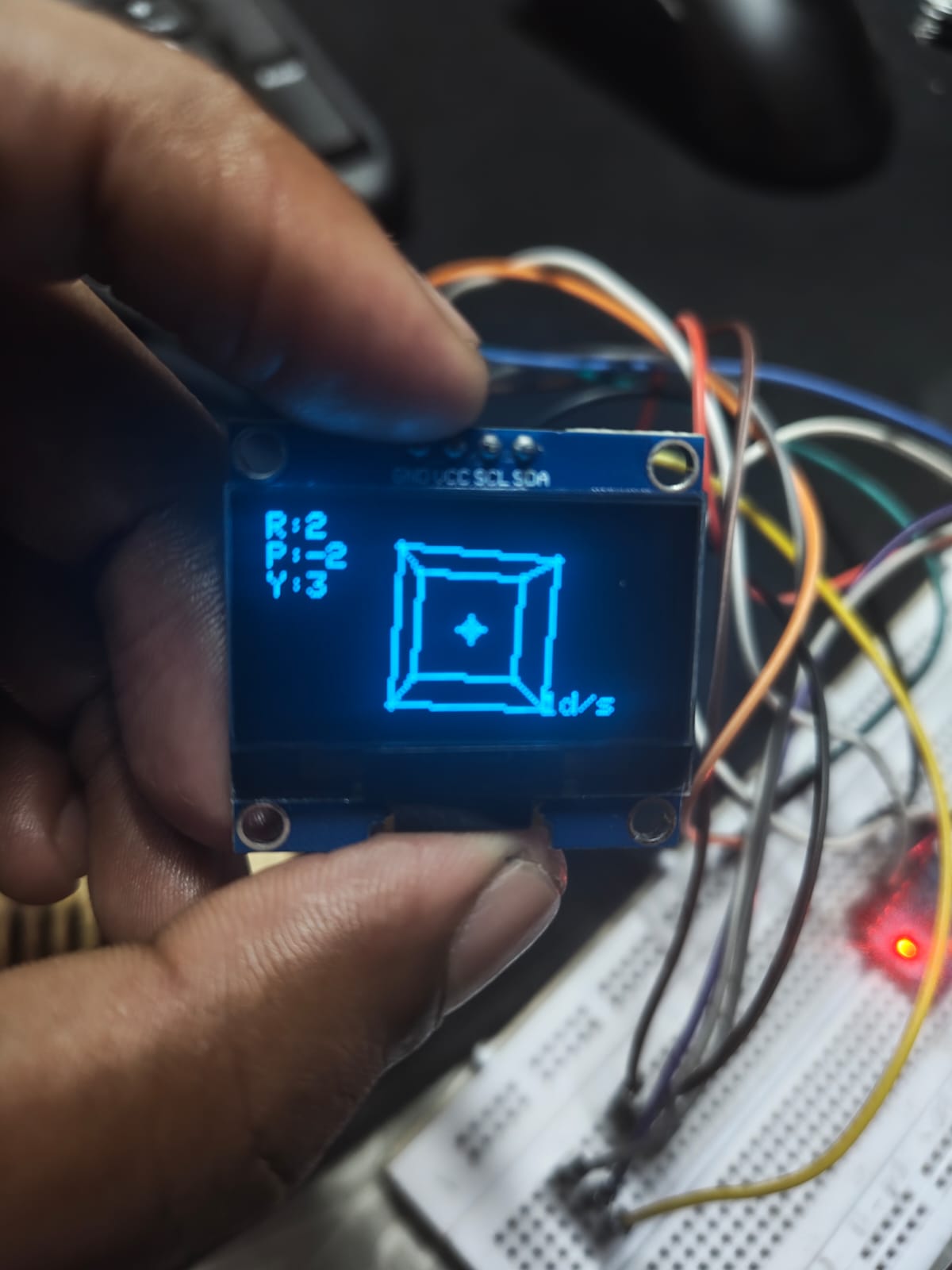
To make the fused orientation verifiable at a glance, I implemented a lightweight 3D graphics rendering engine running directly on the ESP32-S3.
Projection Pipeline
The engine defines a 3D wireframe cube composed of 8 vertices and 12 connecting edges:
- Object Coordinates: 3D vertex coordinates centered at $(X, Y, Z) \in [-s, s]$.
- Euler Rotation: Applying 3D rotation transformation matrices based on the filtered Roll, Pitch, and Yaw angles.
- Perspective Projection: Mapping the 3D rotated points into 2D display coordinates $(x_{\text{screen}}, y_{\text{screen}})$ on the $128 \times 64$ frame buffer: $$x_{\text{screen}} = x_0 + \frac{X \cdot d}{Z + d_z}, \quad y_{\text{screen}} = y_0 + \frac{Y \cdot d}{Z + d_z}$$
- Bresenham Line Rasterization: Drawing the 12 wireframe edges between projected vertices.
- Telemetry Readout: Overlaying live numeric values for Roll, Pitch, and Yaw directly on the display.
This transformed the OLED from a passive output display into an active hardware debugging instrument, allowing direct visual verification between physical breadboard movement and internal state estimation.
🎯 Significance for the TinyML Pipeline
The final objective of this research reproduction is not just displaying orientation angles—it is building an end-to-end predictive maintenance system that detects abnormal motor vibration patterns on resource-constrained microcontrollers.
In the reference research, vibration data is captured at 100 Hz, partitioned into temporal windows, transformed into frequency spectra via Fast Fourier Transform (FFT), and passed into a quantized neural network.
       MPU6050 Sensor
              │
              ▼
   100 Hz Vibration Acquisition
              │
              ▼
       Signal Windowing
              │
              ▼
        16-Point FFT
              │
              ▼
     Feature Extraction
              │
              ▼
       TinyML Model
              │
              ▼
   Edge Anomaly Detection
Establishing this sensing and visualization layer is an essential prerequisite:
- Data Integrity: A neural network cannot compensate for sensor bias, bus dropouts, or incorrect register scale factors.
- Timing & Throughput: Validating that the ESP32-S3 can sample, fuse, and render telemetry in real time confirms that adequate CPU headroom exists for signal processing and neural inference.
- Physical Intuition: Understanding sensor noise characteristics and mechanical coupling prevents spurious anomalies during model evaluation.
💡 Key Takeaways from Part 1
- Data Pipelines Dictate ML Quality: In embedded machine learning, the model is only as reliable as the physical sensing pipeline feeding it. Validating hardware from the bottom up prevents chasing ghost bugs in the ML stage.
- Beware of Library Assumptions: Unexpected register responses like
WHO_AM_I = 0x70highlight the importance of understanding hardware communication protocols directly rather than relying blindly on third-party drivers. - Acceleration $\neq$ Rotation: Visualizing raw data immediately exposed the gravity accumulation issue that would have corrupted orientation estimates.
- Telemetry Accelerates Debugging: Building the 3D wireframe renderer provided an intuitive, real-time feedback loop that validated sensor fusion before moving to complex frequency-domain algorithms.
🚀 Next: Part 2 · Signal Processing
With the sensing layer verified and communicating reliably, the reproduction moves from understanding the sensor to analyzing the vibration signal itself:
- 100 Hz Continuous Sampling: Establishing deterministic timer-driven acquisition.
- Temporal Windowing: Segmenting continuous vibration streams into fixed-size processing frames.
- 16-Point FFT: Transforming time-domain acceleration into frequency-domain spectra.
- Feature Extraction: Computing spectral energy distribution, peak frequencies, and statistical moments for model training.
From there, the extracted features will feed into the on-device TinyML classification engine to detect mechanical anomalies in real time.